Curl and divergence of a vector field

The Curl of a vector field is defined to be

The curl is a measure of the vorticity, or “swirliness”, of the vector field. So imagine that describes some fluid and has the vector field plotted below.

Nykamp DQ, “A rotating vector field.” From Math Insight. http://mathinsight.org/applet/curl_vector_field

Now this field shows that the fluid is rotating in some way around the z axis, this rotation is not what curl measures. To be understand curl, imagine sticking a sphere somewhere in the field and fixing it’s centre, but allowing it to rotate “on the spot”. An applet allowing you to visualise it’s rotation can be found here. Below is a screenshot of it.

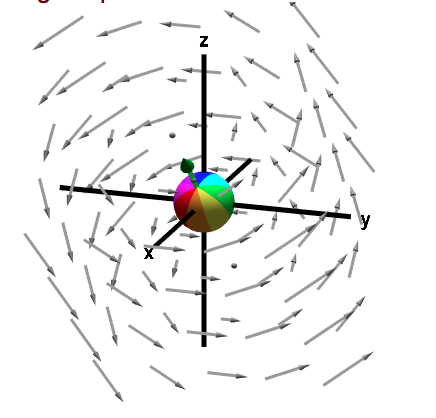
Nykamp DQ, “A rotating sphere indicating the presence of curl.” From Math Insight. http://mathinsight.org/applet/curl_vector_field_sphere_vector

So in this picture, the ball is rotating around the green vector, i.e. the green vector is the axis of rotation. This green vector has magnitude proportional to the speed at which the ball rotates on the spot with. This green vector is precisely the curl! Note that curl only measures how the field “curls” around a point, not how the fluid as a whole rotates.

The divergence of a vector field is defined to be

and is a measure of how the field spreads out from a point. So if you had a large positive divergence at a point, you’re field will point away from the point as shown below, and the point is known as a source.  If you had a negative divergence, the field points into your point and this point is known as a sink.

A physical example of where this is relevant is to do with protons and electrons and their electric fields. Protons will have a large positive divergence while electrons a negative one. Just looking at the above figures, they look similar to the electric fields of protons and electrons.

To summarise, divergence measures spread, curl measures the “curliness” about a point.