A voyage through space(s) (Part I)

So in the last post I talked about wave functions being vectors that live in Hilbert space. In this post, I would like to describe the mathematics of Hilbert space, but before we do that we have to go on a journey, a journey through space(s)!

The first type of space we come across in our journey is a topological space. Say we only know about the set $X$ of natural numbers, $X=\{1,2,3,4,5,6\}$ , for now, and let’s take the following collection of subsets, $T$ :

$T=\{X,\emptyset, \{1,2,3\},\{4,5,6\}\}.$

This collection of subsets of X, is called a topology on X, and we call the pair $(X,T)$ a topological space. We call the sets in T, open sets. (Anything not in T but in X is called closed). However, T isn’t just any random collection of subsets of X; T has three very special properties. First note that $X \in T$ and that $\emptyset \in T$ . Secondly, if we take any union of the sets in T, we get an open set, i.e. the union is in T. Finally, any intersection of the sets in T is still in T. Since T has these three special properties, it is a topology on X. Here is another topology on X

$T=\{X,\emptyset \},$

which is called the trivial topology.

However, in the wild world of maths, we know there are many different non-empty sets. For example we have our standard sets such as $\mathbb{R}, \mathbb{Z}$ and $\mathbb{Q}$ with which we can take any sort of topology that we like. Here is a topological space to mess with your mind: take $X=\mathbb{R}$ and

$T=\{\emptyset,\mathbb{R}\}\cup\{(x,\infty)|x\in\mathbb{R}\}.$

You can prove that (X,T) is a topological space by proving that:

$\emptyset$ and $X$ are indeed open
The union of an arbitrary collection of open sets is open
The intersection of a finite number of open sets is open

Once you have proved that, consider the set $(0,1)$ , is it open? Well, in our standard topology of $\mathbb{R}$ , it is open, however, since $(0,1) \notin T$ , it is closed! Where do we get our standard topology on $\mathbb{R}$ though? How do we define such a collection of sets to be open? Well this leads us onto our next type of space, a metric space.

Now when it comes to a metric space, we still have our large set of things, X, but instead of declaring open sets, we provide some notion of distance between two elements in the set, called a metric. A metric, d, on a metric space X is a function, $d: X^2 \rightarrow \mathbb{R}^+$ such that

$d(x,y)=0 \iff x=y$
$d(x,y)=d(y,x)$
$d(x,y)\leq d(x,z)+d(z,y)$ (Triangle Inequality)

Note here is that the metric takes two elements from our set X (hence why the domain is $X^2$ ) and spits out a positive real number, a distance. The metric space is denoted as $(X,d)$ . Take for example the metric space $(X,d)$ where $X=\mathbb{R}$ and the $d=|x-y|$ . This metric space $(X,d)$ is our standard metric on $\mathbb{R}$ , one you would have been very used to if you have taken any sort of real analysis. However, we can use any sort of notion of distance that we like, as long as it satisfies the three axioms of the metric listed above. Another example of a metric on $\mathbb{R}$ is $d(x,y)=|\arctan{x}-\arctan{y}|$ which can be shown to satisfy the three axioms (try it!).

Now we would really like to know what constitutes an open set in our standard metric on $\mathbb{R}$ , $d=|x-y|$ . But before we can do any of that, we have to get to know some lingo.

Since we want to keep things general for any metric space, we will introduce the lingo in terms of some general metric space $X$ with a general metric $d(x,y)$ .

Imagine I pick a point $a$ that lives inside my metric space $X$ , that is $a \in X$ . Now I want a way to distinguish between points that are close to it and those that aren’t. One way I can do this is by drawing a circle around it of radius of $r$ .

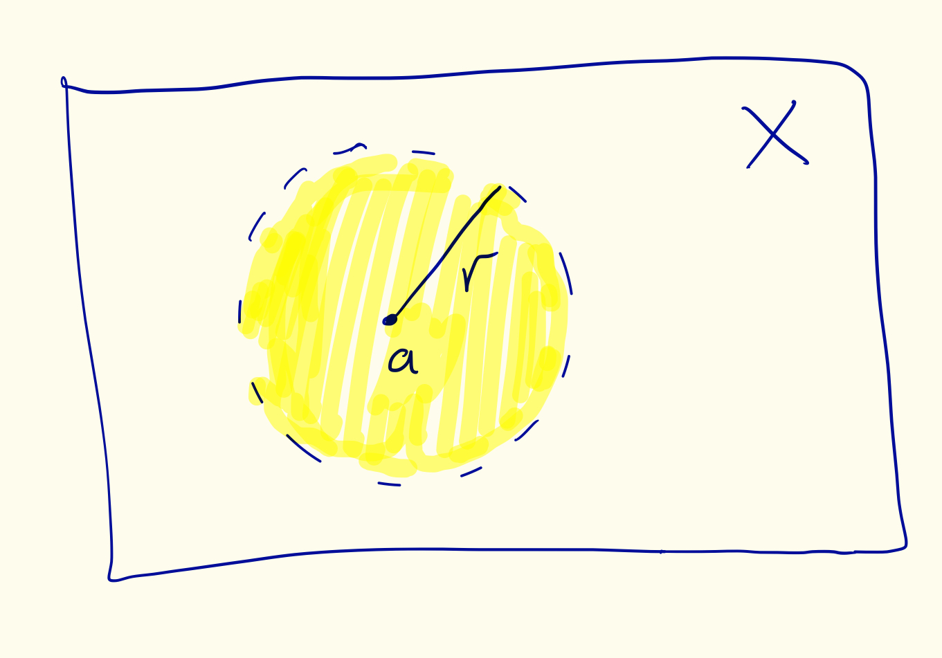
Every point $x$ inside the circle (yellow) are within distance $r$ to $x$ , specifically, $d(a,x)<r$ . That yellow region is called the open ball centred at $a$ with radius $r$ and the way we write this is $B(a;r)$ . Now for some more words.

Say I have a set $A \subset X$ .

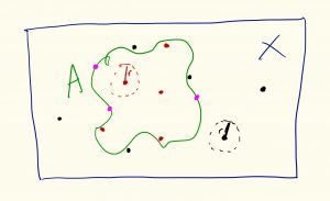
Now there are three possible ways a point in $X$ can be related to $A$ . It can be either in $A$ (red), not in $A$ (black) or on the boundary of $A$ (pink).

The red points are interior points, which means I can find a small enough radius $r$ such that the open ball centred at the red point x, $B(x;r)$ , is completely inside $A$ , that is $B(x;r)\subset A$ .

The black points are called exterior points which means I can find a small enough radius $r$ such that the open ball centred at each black point, $x$ , $B(x;r)$ is completely outside $A$ , that is, $B(x;r)\subset X \setminus A$ .

The rest of the points are called boundary points.

The set of all points inside $A$ (the interior) and all the points on the boundary is called the closure of $A$ , $\bar{A}$ .

So the set $X$ is split into three parts, the interior $A^\mathrm{o}$ , the exterior $\bar{A}^c$ and the boundary. Now that we have this arsenal, we are ready to tackle what an open set is.

A set A is open if $A=A^\mathrm{o}$ . That is, all the points of A are interior points, meaning A does not contain it’s boundary. As usual a set F is closed if it’s complement, $X\setminus F$ is open in $X$ . We can now see that using our standard metric on $\mathbb{R}$ , the set $(0,1)$ is open because it doesn’t contain its boundary.

Just like we have sets, sequences, series and functions in $\mathbb{R}$ , we can have all the same things in any metric space X. What we want to look at now are sequences in any sort of metric space $(X,d)$ . Just like a sequence of real numbers we have a definition of convergence which states that a sequence $x_n$ in a metric space $X$ converges to a limit $x$ when

$\forall \epsilon>0, \exists N, n \geq N \implies d(x_n,x)<\epsilon.$

This just means that no matter how small I make my ball around x, I will always have other points of my sequence $x_n$ contained within that ball. But as usual, this definition is circular, it requires us to know what the limit is. So we have the notion of a Cauchy sequence in a metric space which is a sequence $x_n$ where the elements get arbitrarily close together, that is

$d(x_n,x_m)\rightarrow 0, \text{as}~~ n,m\rightarrow \infty.$

Now we know that everything from real analysis applies to our standard metric on $\mathbb{R}$ , so let’s keep our space as $\mathbb{R}$ but use the metric defined previously as $d(x,y)=|\arctan(x)-\arctan(y)|$ . Take for example the sequence $x_n=n$ , and let us see what happens between any two points in the sequence as $n\rightarrow\infty$ . We know that $\arctan(n)\rightarrow\frac{\pi}{2}$ as $n\rightarrow\infty$ , so this means that $d(x_n,x_m) \rightarrow 0$ as $n,m \rightarrow \infty$ . So our sequence $x_n=n$ is Cauchy! But this means that we have a Cauchy sequence that doesn’t converge, which is very different from real analysis. So unlike real analysis, we can have sequences in our metric spaces that are Cauchy that do not converge!

This may all come as a shock to you, but I am like Morpheus and you Neo, and you have two pills in front of you. You take the blue pill, the story ends. You wake up in your bed and believe whatever you want to believe. You take the red pill, you stay in wonderland, and I show you how deep the rabbit hole goes. It’s up to you. If you take the red pill, stay tuned for my next post.

A voyage through space(s) (Part I)

Like this:

Related

1 Comment

Leave a Reply to Ivan Cancel reply

Recent Posts

Recent Comments

Archives

Categories

Subscribe to Blog via Email

A voyage through space(s) (Part I)

Share this:

Like this:

Related

1 Comment

Leave a Reply to Ivan Cancel reply

Recent Posts

Recent Comments

Archives

Categories

Subscribe to Blog via Email