So these spaces are really interesting, but super duper hard to get your head around. So in this blog, I hope to make there equivalent definitions a little bit easier to understand.

I’m going to present 3 equivalent definitions of the n-dimensional real projective space using the language of quotient spaces, and then prove that they are indeed equivalent.

A. is by identifying the antipodal points. (Sphere Model)

B. is by identifying two points if they lie on the same line through the origin. (Line Model)

C. is the unit ball and identifying antipodal points on its surface. (Ball Model)

Now all three models are quotient spaces, and to prove that they are equivalent, i.e. that they are homeomorphic, we will need a bit of theory about identification maps. So let’s take a few moments to say a couple of things.

Say, we have topological spaces and , and a continuous surjective map , then we call an identification map. Why? Because, provides a natural partition of the space into subsets where . That might boggle your mind, so let’s take a look at an example.

Consider the spaces and . We can define the continuous surjective function

   

Now, clearly, any vector that points in the same direction in will get mapped to the same point on . These sets of pre-images of the point provide the partition of , known as the sets of the pre-images of f, . We can see now, that we can describe as the disjoint union of the pre-images of , i.e.

   

Since is surjective, none of these sets will be the empty set and so it is well defined. Now, we can represent this quotient space as , which reads as partitioned into pre-images of .” Now, in the example I chose, it is obviously true that is homeomorphic to .

Now let’s go back to the general case, topological spaces and and the map . Now if is an identification map, it immediately follows that is homeomorphic to , i.e. that in the picture below is a homeomorphism. Also note, that the is just the canonical projection form to it’s quotient space.

Now, there are two results that we can use to check if our given map is an identification map, and then simply state that and are homeomorphic, let’s state them so we can use them. The first result relates to the map and the second one relates to the spaces.

Theorem 1: If a surjective and continuous map maps open sets to open sets, or closed sets to closed sets, then is an identification map.

Theorem 2: Let be a surjective and continuous map from to . If is compact and is Hausdorff, then is an identification map.

Now we have the necessary gadgets to prove that the three definitions of the real projective space are indeed homeomorphic. Let’s start by showing that the sphere model is homeomorphic to the line model, and it is always a good idea to draw out a little diagram of our spaces and what maps what to what.

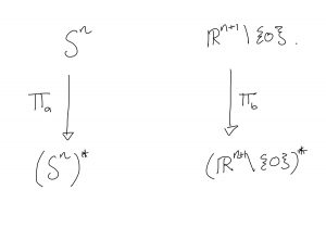
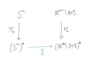
Now, we want to show that the bottom two spaces, are homeomorphic, so following the general model that we introduced above, we want to be between them.

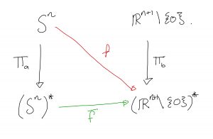
So this must mean we need to find an identification map between the diagonal spaces, shown in red below.

Now, we can try really hard to be smart and think of a single map straight to , or we can just compose some simple functions. Namely, we can see that we can go from to using the inclusion map.

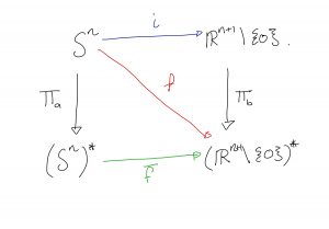
Now since and are both continuous and surjective, it follows that is also continuous and surjective. is a closed subset of and is therefore compact. We now just need to show that is indeed Hausdorff and we would be done by Theorem 2.

So now,  let’s prove that this space is Hausdorff. This is no small feat. The idea behind this will be to use the fact that we can find disjoint open sets in because it is Hausdorff, and then use our quotient map to take these disjoint open sets to disjoint open sets in the quotient space.

So we start by taking two elements and in our quotient space, which are just lines through the origin in . We can look at the intersection of these lines with , which would be 4 distinct points, are the intersections of with , and are the intersections with . Since is a subset of the Hausdorff space , we can find disjoint open sets that contain each of and  , call them and . Furthermore, we can construct each of these sets so that if then , which ensures that , and the same for . Now, for any , it follows that , hence, , which ensures that . Now, don’t let this trip you out, we only need to have a little bit of the line in , so that in the quotient space, contains the equivalence class , and same for and . So, in the quotient space, and is open, and and is open. Hence, is Hausdorff!

Now, we want to show that Ball Model in C, is equivalent to the sphere model in A. Here is the map of our spaces and functions.

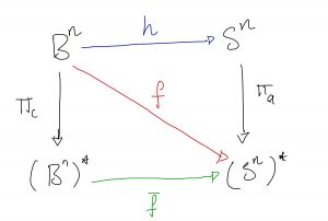
Where takes the point to . Clearly, is continuous and surjective, and so the is continuous and surjective. Now, clearly is compact, and is Hausdorff, the proof of which is virtually the same as that above just ignore the lines through the origin business and go straight to antipodal points. It follows that is an identification map and so is homeomorphic to .

Brace yourself,

You’re probably thinking, what the heck is the point of all this, like why on earth are we even doing this? Other than for the pure joy of it, which is of course enough of a reason to do it, there is a really nice connection between the projective plane, , and non-orientable surfaces. We will build up to understanding this and then we will come back to our beloved projective plane .

So, what the hell is a surface? You probably have an idea what a surface is, you might think it’s a shape in 2 or 3 dimensions that has some faces, edges and vertices. Well, this is what comes to my mind when I think of a “surface”. But, what isn’t so natural to think of is how we work mathematically with surfaces, however, you’re in luck, because it is quite intuitive. We know that a surface is made up of vertices, edges and faces. So we would like to define these building blocks as simplicies. So, consider a rectangle, it has 4 vertices as shown, 4 edges and 1 face which are called the 0-simplex, 1-simplex and 2-simplex respectively.

Now, here I’ll stop and introduce something pretty neat, called the Euler characteristic of surface which is

   

In terms of our everyday language, this is just vertices – edges + faces. Take note of this, it’s gonna come back big time.

Finally, we note that we can give a surface an orientation, which is an ordering of the vertices. If the faces of the surfaces can be orientated such that a loop on the face going clockwise cannot be continuously deformed to a loop going anti-clockwise without overlapping itself, we say that the surface is orientable. As an example, consider the Mobius strip, it is non-orientable as a loop on the boundary goes clockwise and then anti-clockwise. In fact, if a surface contains a subset homeomorphic to the mobs strip, it is not orientable.

Here we go,

Now, it turns out, that any connected non-orientable surface, is homeomorphic to the connected sum of n-projective planes . WHAAAAAT! Completely unexpected, right!?

But how do we know how many projective planes we need? Well, we look at the Euler characteristic of course!

Th Euler characteristic of the connected sum of n projective planes is

   

Now all you need to do is figure out, how many projective planes you need to get the same Euler characteristic of your surface, and bam, you done.

As a side note, if the surface is orientable, it is the connected sum of n-tori or it is the sphere if , where for the connected sum of n-tori.

Now, why is this so useful? Because once you know what you’re homeomorphic to, you can easily compute the fundamental group of connected sums of the projective plane.

So there you go, any surface, is exactly the same as either a sphere, the connect sum of n-tori or the connected sum of n-projective planes. What a time to be alive.